I. Solution Overview
For chip-level MEMS gyroscopes/IMUs (primarily the gyroscope channels), the difficulty in performance evaluation and calibration is often not “being able to measure data”, but rather “controllable input conditions, consistent and traceable data, a unified calculation convention, and reproducible conclusions”. Therefore, this note proposes an automated test solution for chip-level MEMS gyros/IMUs, aiming to standardize the test process and deliver results with one click.
The system consists of a data acquisition and analysis system, automated test software, an angular vibration table, a dual-axis position table, and an integrated rate table built into a temperature chamber. It can cover key static, dynamic, and temperature-related metric tests. The data acquisition and analysis system serves as a unified acquisition and control platform, providing multi-channel synchronous acquisition, long-duration logging, and basic time-domain/frequency-domain analysis; the automated test software runs on the acquisition system to enable coordinated control of the fixtures, test-sequence orchestration, automatic data processing, metric calculation, and report output. The rate table inside the temperature chamber provides stable angular-rate stimuli under temperature control for scale factor and derived items, threshold/resolution, temperature sensitivity/temperature drift, etc. The dual-axis position table provides precise attitude flips for bias acceleration sensitivity (g-sensitivity). The angular vibration table provides controllable angular vibration stimuli for amplitude/phase frequency response, bandwidth, and other dynamic metrics. The test system architecture is shown below:
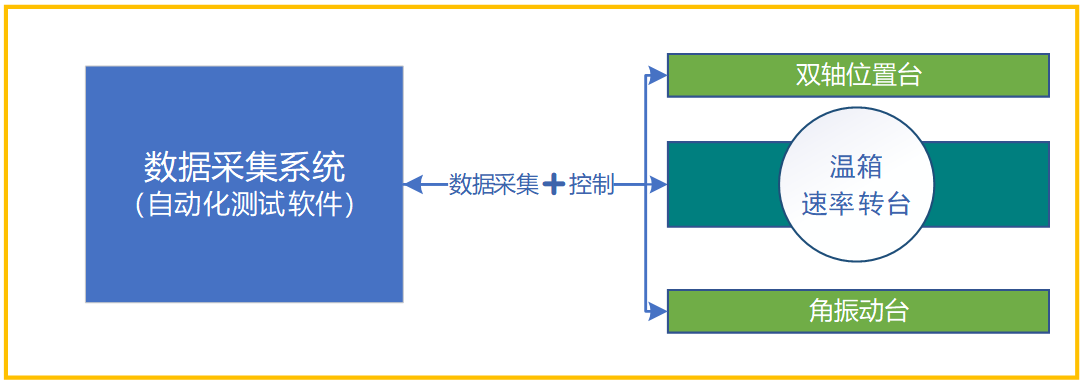
During testing, the DUT gyroscope chip is mounted on the fixture and connected for power and signal. The software controls the fixtures to apply stimuli such as angular rate, angular vibration, attitude, and temperature; the acquisition system synchronously captures the gyroscope outputs and logs them over a long duration. After the test, the software automatically processes the data and computes the metrics, provides conclusions, and outputs a report.
2. Test Basis
2.1 Reference Standard
This solution targets performance testing and calibration of chip-level MEMS gyroscopes/IMUs (primarily the gyroscope channels). A specification that systematically defines the “test items, test methods, and result expression” is needed as the technical backbone. JJF 1535—2015, Calibration Specification for Micro-Electro-Mechanical (MEMS) Gyroscopes, establishes a complete calibration framework for MEMS gyroscopes: in scope, it focuses on single-sensing-axis MEMS gyroscopes and provides executable guidance that can be referenced for multi-axis devices; in content, it standardizes key chip-level performance metrics and specifies corresponding calibration/test methods and requirements for result reporting.
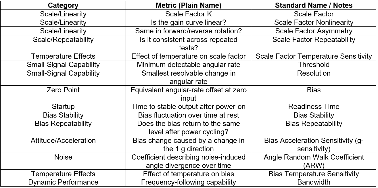
The specification covers the core performance elements for chip-level testing, including: scale factor and its nonlinearity, asymmetry, and repeatability; bias and its stability and repeatability; bias temperature sensitivity and bias acceleration sensitivity; angle random walk (ARW) and bandwidth, etc. These metrics directly characterize a MEMS gyroscope’s static accuracy, noise level, environmental sensitivity, and dynamic response. Meanwhile, the specification provides explicit recommendations on calibration environmental conditions and key equipment configurations (e.g., rate table, temperature chamber, angular vibration device, and position device, and their recommended performance), making it easier to form a consistent engineering implementation path for system configuration, equipment selection, and test-flow design.
In summary, JJF 1535—2015 is suitable as the primary reference standard for the chip-level MEMS gyroscope/IMU test system in this solution. If the test scope is later extended to higher environmental stress conditions or module-level devices (e.g., high-grade IMU modules, FOG/HRG modules, etc.), corresponding environmental/reliability standards and module-level test specifications can be added on this basis to meet the applicability requirements of the extended scenarios.
2.2 Test Metrics
3. Key Test Equipment
3.1 Data Acquisition and Analysis System
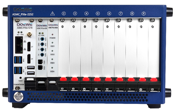
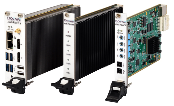
In the rate-table calibration and frequency-response calibration sections, JJF 1535—2015 recommends supporting instruments such as a 6½-digit voltmeter (frequency counter), a spectrum analyzer covering 1 Hz–10 kHz, and a 20 MHz oscilloscope for output measurement, spectrum/waveform observation, and recording. This solution uses a PXIe-based modular data acquisition and analysis platform, integrating control, acquisition, and storage in the same chassis. With a unified timebase and synchronous acquisition, it ensures consistent multi-channel logging and provides frequency/period measurement and FFT spectrum analysis in software, thereby equivalently covering the “frequency counter / spectrum analyzer / oscilloscope” functions required by the standard.
A typical configuration is: PXIe chassis + embedded controller + high-speed storage card, supporting long-duration continuous recording and data replay for recalculation. The chassis provides 10 MHz clock I/O to share a common timebase and enable extended synchronization with systems such as the rate table, temperature control, and position table. Acquisition cards are selected based on the DUT output type (analog / frequency / digital), covering time-domain observation, statistical mean/dispersion calculations, and frequency-domain analysis needs.
3.2 Rate Table and Temperature-Control System (Integrated Temperature Chamber / Temperature-Controlled Rate Table)
The rate table is the core standard fixture for scale factor and derived items (nonlinearity, asymmetry, repeatability), as well as threshold, resolution, and more. JJF 1535—2015 recommends an angular-rate accuracy and steadiness of 0.05% (for rates > 10°/s), and a temperature chamber for temperature-sensitivity-related items. Recommended chamber performance: temperature deviation ±2 °C, temperature fluctuation 1 °C, and temperature uniformity 2 °C.
In engineering implementation, this solution prioritizes an integrated structure such as a rate table built into a temperature chamber or a temperature-controlled rate table, so that “angular-rate stimulation + temperature environment” can be stably established under the same conditions, reducing error sources introduced by transfer and re-fixturing. Meanwhile, the acquisition system performs output sampling and point-data management to ensure that subsequent least-squares fitting and statistical calculations are traceable.
3.3 Dual-Axis Position Table (Flip Table)
The dual-axis position table is used for calibrating bias acceleration sensitivity (g-sensitivity). JJF 1535—2015 recommends an angle-position accuracy of ±3″ and an angle-position measurement repeatability of ±3″, along with a 6½-digit voltmeter (frequency counter) for output measurement. In this solution, the acquisition system performs static sampling, mean calculation, and automatic archiving of data across attitude changes. It supports generating a standardized dataset following the 6-attitude procedure of “X/Y/Z axis pointing up, in both positive and negative directions”, making it convenient to compute the g-sensitivity for each axis per the specification and take the maximum as the reported result.
3.4 Angular Vibration Table (Frequency-Response Calibration Fixture)
The angular vibration table is used for calibrating amplitude-frequency response, phase-frequency response, and bandwidth. JJF 1535—2015 recommends a waveform distortion ≤ 2%, and suggests supporting instruments including a spectrum analyzer (1 Hz–10 kHz), a 20 MHz oscilloscope, and a 6½-digit voltmeter (frequency counter).
In the measurement chain, this solution uses the acquisition system to synchronously capture both the angular-vibration input reference and the gyroscope output, extract amplitude and phase, and fit the frequency-point curves. This meets the standard’s requirements for spectral analysis and phase measurement across 1 Hz–10 kHz, and produces reproducible raw records and processed-result files to support end-to-end traceability for bandwidth (-3 dB) determination.
3.5 Automated Test Software
JJF 1535—2015 clearly specifies the calibration items and calculation methods. On this basis, this solution adds automated test software to centrally orchestrate the rate table, temperature control, position table, angular vibration table, and acquisition system. It solidifies the test sequences and data-processing flows, automates generation of rate points/frequency points, automates sampling and statistics, and automates metric calculation and report output—reducing operator variability and improving test consistency.
4. Example Test Methods
4.1 Test Preparation
1. Environment check: temperature (20 ± 5) °C; temperature fluctuation during calibration ≤ 2 °C; humidity ≤ 85%; no strong electromagnetic fields / corrosive media / strong vibration sources nearby.
2. Confirm DUT gyroscope information: model, range, output type (voltage / frequency / digital), power requirements, communication, and sampling method.
3. Check connections: verify power, signal wiring, grounding, and shielding; confirm the host PC/recording software can sample and store data reliably.
4. Warm-up: per the specification, power-on warm-up is typically ≤ 30 min; use output stability as the criterion.
5. Unified logging: for each test, record the date, environment, equipment ID(s) / calibration validity, sampling settings, attitude/axis, input points, and raw data filenames.
Module A: Multi-Point Sampling on the Rate Table (for K and Derived Items)
Purpose: use a set of “known rate points” to fit the relationship between output and input, obtain the scale factor K, and derive nonlinearity, asymmetry, repeatability, etc.
1. Installation: mount the gyroscope on the rate table, with the input reference axis pointing upward (aligned with the rate-table rotation axis).
2. Sampling setup: verify cable connections; start the rate table; recommended sampling period is 1 s (or as required).
3. Warm-up: power the gyroscope and warm up (typically no more than 30 min) until the output stabilizes.
4. Point planning: select rate points within the measurement range (≥11 points forward and ≥11 points reverse, both including the maximum input angular rate; points should be as evenly distributed as possible; you may reference the R5 preferred-number series in GB/T 321 to select candidate points, then round and/or delete points as needed).
5. Point-by-point sampling: change the input angular rate sequentially according to the point list; after the table stabilizes at each point, sample and record the output. For points with |rate| < 100°/s, take ≥30 samples per point; for points with |rate| ≥ 100°/s, take ≥5 samples per point.
6. Two zero-rate measurements: at the start and end of calibration, stop the rate table (0°/s) and measure the mean output once each; later, remove it from the mean output at each rate point to reduce the impact of bias on K.
7. Repeat: as needed, repeat the entire procedure after a period (e.g., re-test after 30 min) to evaluate repeatability/stability.
8. Computation: compute the mean output at each point; use least squares to fit “Output = K × Input + fitted zero”, obtaining K (slope).
Tip: if the output is frequency or digital codes, the idea is the same—the essence is a linear fit between the input points and the mean outputs.
Module B: Static Sampling (for Bias / Readiness Time / Stability / ARW, etc.)
Purpose: continuously sample at “input angular rate = 0” to obtain the bias and its time-varying behavior.
1. Installation: mount the gyroscope on the calibration base using the fixture, with the input axis perpendicular to the base (fixed attitude).
2. Warm-up: apply power and warm up (typically no more than 30 min) until the output stabilizes.
3. Sampling setup: set the sampling interval and total duration (recommend at least tens of minutes; longer is recommended for ARW).
4. Start logging: keep the gyroscope completely stationary; continuously record the output and save the raw data.
5. Compute bias: average the sampled output, then convert to equivalent angular-rate bias using K (B0 = mean output / K).
6. For repeatability: power off → wait → power on → warm up, then repeat the sampling above and run multiple trials for statistics.
4.2 Example Detailed Test Procedures
1. Scale Factor K
Equipment: Rate Table + Acquisition/Logging System
Procedure:
1. Execute Module A end-to-end: installation & alignment → warm-up → point selection → point-by-point sampling → two zero-rate measurements → (optional) repeat measurement.
2. For each input angular-rate point, compute the mean output (with the zero-rate contribution removed).
3. Fit K via least squares (the slope of the output–input line).
Results / acceptance: Build an input–output linear model by least squares, Fj = K·Ωij + F0 + vj, where K is the slope of the fitted line (scale factor), F0 is the fitted zero, and vj is the residual. The output should include at least K, F0, and residual statistics (e.g., maximum residual, RMS, etc.), and retain the mean outputs and point list for each calibration point for subsequent nonlinearity and asymmetry calculations. If repeated calibration is performed per the specification (Q runs), statistical results for K (mean and dispersion) should be reported.
2. Scale Factor Nonlinearity
Equipment: Rate Table + Acquisition/Logging System
Procedure:
1. Reuse the same dataset from Module A, or re-acquire data following Module A.
2. Use the fitted line to compute the theoretical output at each point, and subtract the measured mean.
3. Find the maximum deviation and normalize it using the standard formula (i.e., maximum deviation as a proportion of the full-scale input range).
4. If multiple repeats are performed, take the average as the final result.
Results / acceptance: Using the same set of calibration points, compute the deviation between the fitted-line output F̂j and the measured mean Fj at each point. Take the maximum deviation and normalize it to the full-scale input range per the specification to obtain the single-run nonlinearity K′m. If calibration is repeated Q times, average K′m per the specification to obtain K′. The output should include K′ (or the K′m series), the point corresponding to the maximum deviation, and the parameters used for normalization such as Ωmax+ and Ωmax−.
3. Scale Factor Asymmetry
Equipment: Rate Table + Acquisition/Logging System
Procedure:
1. Acquire two datasets (forward and reverse rotation) following Module A.
2. Fit the forward-rotation data to obtain K+, and fit the reverse-rotation data to obtain K−.
3. Use the standard formula to compute the difference between K+ and K− relative to their mean.
4. If multiple repeats are performed, take the average as the final result.
Results / acceptance: Fit the forward- and reverse-rotation datasets to obtain K+ and K−, respectively. Compute, per the specification, their difference relative to the mean scale factor K̄ to obtain the single-run asymmetry Kmu. If calibration is repeated Q times, average Kmu to obtain Ku. The output should include K+, K−, K̄, and Ku (or the Kmu series).
Doewe Technology has always been committed to delivering innovative, distinctive, and reliable product solutions in the data acquisition field. We understand that these elements are the foundation for companies to stay competitive. For this reason, our innovation is inspired by real customer application needs—not merely by eye-catching but impractical product features. By continuously optimizing and enhancing DAQ solutions, Doewe Technology helps partners move toward a more efficient and precise future. Choose Doewe Technology, and join us in opening a new chapter in data acquisition.